What is a T-Test? Types, Assumptions, and Calculations Explained
Let’s be honest for a moment. For many of us in the mental health field, the word “statistics” triggers a mild fight-or-flight response. We entered this profession to understand the human mind, to help people navigate trauma, and to foster growth, not necessarily to crunch numbers.
However, statistics is the bridge between a hunch and a scientific fact. It is the tool that tells us if a new therapy actually reduces depression or if a medication is truly effective.
One of the most fundamental tools in our research toolkit is the T-test. If you have ever wondered how researchers determine if two groups are actually different from one another, or just look different by chance, this is the method they use.
In this guide, I am going to break down the T-test based on clear, educational insights. We will cover what it is, the three specific types you need to know, and how to make sense of the results without getting a headache.
What is a T-Test?
At its core, a T-test is a statistical procedure used to determine if there is a significant difference between the means (averages) of two groups.
Think about it this way: If you measure the blood pressure of two different groups of patients, the average scores will rarely be exactly the same. But is that difference meaningful? Or is it just random noise? The T-test analyzes this variance to give us a clear answer.
The Basic Function
The T-test looks at the data and calculates a ratio. It compares the difference between the two groups against the variation within the groups (the standard error). If the difference between the groups is large compared to the scatter of data inside the groups, we likely have a significant result.
The Three Types of T-Tests
Not all research questions are the same, so we have three different versions of this test to handle different scenarios. Choosing the right one is critical for valid results.
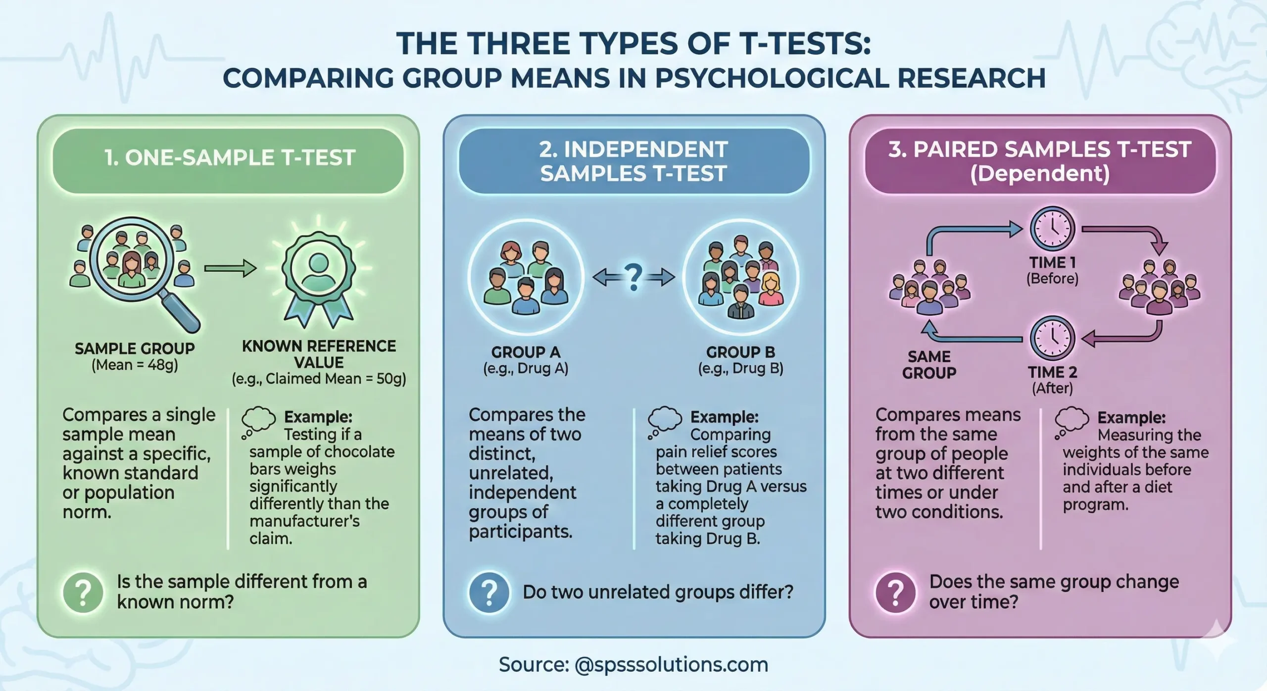
1. The One-Sample T-Test
We use this when we want to compare the mean of a single sample against a known reference mean or a population norm.
The Chocolate Bar Example: Imagine a manufacturer claims their chocolate bars weigh exactly 50 grams. You want to test this. You grab a sample of 30 bars and weigh them, finding the average is actually 48 grams.
The Question: Is that 2-gram difference just a fluke, or is the manufacturer’s claim wrong?
The Test: The One-Sample T-test compares your sample mean (48g) against the specific reference value (50g) to see if they differ significantly.
2. The Independent Samples T-Test
This is one of the most common tests in psychological research. We use it when comparing the means of two independent, unrelated groups. “Independent” simply means that the people in Group A are completely different people than those in Group B.
The Painkiller Experiment: Let’s say we want to compare the effectiveness of Drug A versus Drug B. We randomly assign 60 participants into two groups. Group 1 gets Drug A; Group 2 gets Drug B.
The Question: Is there a significant difference in pain relief between the two distinct groups?
The Test: Because the participants in Group 1 have no relationship to those in Group 2, we run an Independent Samples T-test.
3. The Paired Samples T-Test (Dependent T-Test)
We use this when comparing means from the same group of people at two different times or under two different conditions. The data points are “paired” because they come from the same source.
The Diet Study: Suppose we want to evaluate a new diet plan. We weigh 30 people before they start the diet, and then we weigh those exact same 30 people after the diet.
The Question: Did the participants’ weight change significantly from Time A to Time B?
The Test: Since the measurements are dependent (the same person provides both the before and after score), we use the Paired Samples T-test.
Psychologist’s Note: You can think of a Paired T-test as a variation of the One-Sample test. Essentially, we calculate the difference for each person (After minus Before), and then test if the average of those differences is significantly different from zero.
Assumptions: The Rules of the Game
Before you hit “calculate” in your statistical software, you must ensure your data follows certain rules, known as assumptions. If you violate these, your results might be misleading.
Metric Variables: The variable you are measuring (e.g., weight, blood pressure, anxiety score) must be metric (interval or ratio scale). Categories like “Education Level” are ordinal and do not work here.
Normal Distribution: Your data should roughly follow a bell curve. However, T-tests are fairly “robust,” meaning they can handle slight deviations from normality if your sample size is decent (usually more than 30 people per group) and you don’t have extreme outliers.
Homogeneity of Variance: For the Independent T-test, the variance (how spread out the scores are) should be roughly equal in both groups. You can check this using Levene’s Test.
Hypothesis Testing: Null vs. Alternative
In statistics, we always start with a skeptic’s mindset.
The Null Hypothesis (H0): This is the assumption that nothing is happening. It states that the means are equal. (e.g., “There is no difference between Drug A and Drug B”).
The Alternative Hypothesis (H1): This states that there is a difference. (e.g., “The means of the two groups are not equal”).
Our goal with the T-test is to see if we have enough evidence to reject the Null Hypothesis.
Calculating and Interpreting the Results
When you run the test, you get a T-value.
Large T-value: Indicates a large difference between groups relative to the spread of the data (the signal is stronger than the noise).
Small T-value: Indicates the difference is likely just random variation.
The P-Value
The T-value helps us find the p-value, which is the star of the show.
If p < 0.05: The result is statistically significant. We reject the Null Hypothesis. We are saying there is less than a 5% probability that this result occurred by chance.
If p > 0.05: The result is not significant. We stick with the Null Hypothesis.
A Real-World Interpretation Example
Let’s look at the blood pressure data from our previous example.
Null Hypothesis: No difference between Drug A and B.
Result: You run the Independent T-test. The p-value comes back as 0.03.
Conclusion: Since 0.03 is smaller than 0.05, we reject the Null Hypothesis. We can confidently say that Drug A and Drug B produce significantly different results in lowering blood pressure.
Conclusion
Statistics might feel like a foreign language at first, but concepts like the T-test are actually quite intuitive once you strip away the formulas. Whether you are looking at chocolate bars, blood pressure, or therapy outcomes, the logic remains the same: we are comparing averages to see if a difference is real.
Mastering these basics does more than just help you pass a class. It empowers you to read psychological literature critically. When you see a claim that “Treatment X is better than Treatment Y,” you will know exactly what evidence is required to back that up.
Reflection: Think about a behavior or trait you have observed in your daily life. If you wanted to test if it differs between two groups (like early birds vs. night owls), which of the three T-tests would you use?