Empirical CDF (ECDF): Definition, Properties, Computation, and Applications

In statistics, the cumulative distribution function (CDF) describes the probability that a random variable takes a value less than or equal to a given point. While theoretical CDFs rely on assumed distributions (such as normal or exponential), real data seldom follow a perfect model. The empirical cumulative distribution function (empirical CDF or ECDF) is a non-parametric estimator of the true CDF, built directly from sample data. This post explains the formal definition of the empirical CDF, its properties, how to compute and plot it in different software (including SPSS), and why it is a powerful tool for researchers and data analysts.

Table of Contents

Definition of Empirical CDF

Given a sample X1,X2,…,Xn drawn from an unknown distribution, the empirical CDF at a point xxx is defined as:

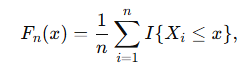
where I{⋅} is an indicator function (1 if the statement is true, 0 otherwise). In plain terms, Fn(x) is the proportion of observations less than or equal to xxx in your data. It is a step function that jumps by 1/n at each observed data point (or by more if there are ties).

Key properties (StatLect, 2024):

Non-decreasing and right-continuous.
Range: from 0 to 1.
Consistency: by the Glivenko–Cantelli theorem, the empirical CDF converges uniformly to the true CDF as nnn increases (Wikipedia, 2024).
Unbiased at fixed x: its expected value equals the true CDF at that point.

These properties make the ECDF a fundamental non-parametric tool in statistics.

How to Compute and Plot an Empirical CDF

The procedure is simple:

Sort your data from smallest to largest.
Count cumulative frequencies: for each unique value xxx, compute #{Xi≤x}/n.
Plot x on the horizontal axis and Fn(x) on the vertical axis. The result is a staircase-like graph.

Software Implementation

R: ecdf(x) creates an ECDF function; plot(ecdf(x)) plots it.
Python (statsmodels):
from statsmodels.distributions.empirical_distribution import ECDF
ecdf = ECDF(data)
plt.step(ecdf.x, ecdf.y)

Or use seaborn’s sns.ecdfplot(data).
SPSS: Although SPSS does not have a direct “ECDF” command, you can obtain cumulative percentages through Analyze > Descriptive Statistics > Frequencies and then plot the cumulative percent values (Graphs > Chart Builder). This produces a visual empirical CDF of your variable.

Including these code snippets enhances reproducibility and makes the concept more concrete for readers.

Interpreting an Empirical CDF Plot

An ECDF plot shows on its x-axis the observed data values and on its y-axis the cumulative proportion (percentile). It allows you to:

Determine the data range (first and last steps of the function).
Identify where most values occur (steeper steps indicate denser regions).
Estimate percentiles: for a given value, read its percentile on the y-axis; for a given percentile, draw a horizontal line to see the corresponding value.

Unlike Q–Q plots, ECDF plots are not transformed to produce straight lines. They display the data’s cumulative structure directly and can be overlaid with a fitted CDF to assess goodness-of-fit (Statistics by Jim, 2024).

Applications of the Empirical CDF

Estimating Percentiles and Quantiles: The ECDF directly gives you the empirical percentile of any observed value.
Comparing Distributions: Overlaying ECDFs of two or more samples visually highlights differences in location, spread, and skewness. For instance, in quality control or treatment studies, ECDF plots can show which group has lower variability or higher performance.
Goodness-of-Fit Testing: Tests such as the Kolmogorov–Smirnov and Cramér–von Mises rely on the ECDF to compare observed data against a theoretical distribution.
Outlier Detection: Extreme values manifest as large jumps at the tails of the ECDF.
Non-parametric Inference: Because the ECDF makes no assumptions about the data’s distribution, it is widely used in robust statistics, economics, and psychology research.

Confidence Bands and Asymptotic Behavior

While an ECDF shows the estimated CDF, sampling variability means it is only an approximation. Confidence bands quantify this uncertainty. The Dvoretzky–Kiefer–Wolfowitz (DKW) inequality provides a nonparametric bound for how far the ECDF can deviate from the true CDF uniformly. As the sample size increases, the ECDF becomes smoother and converges uniformly to the true CDF. In practice, larger samples yield more reliable ECDF estimates and narrower confidence bands (Massart, 1990).

Limitations and Practical Considerations

Step Function Nature: With small samples, the ECDF may look jagged. For smoother curves, some analysts prefer kernel smoothed CDFs.
Handling Ties: Tied observations cause jumps larger than 1/n1/n1/n, which is correct but must be interpreted carefully.
Computational Load: For very large datasets, computing and plotting ECDFs requires efficient algorithms, but most statistical software handles this easily.
Model vs. Empirical: A fitted (parametric) CDF may be smoother but depends on assumptions; the ECDF is assumption-free but reflects sample variability.

Example: Using an Empirical CDF in Practice

Suppose you have test scores for 200 students. By plotting the ECDF you can:

Identify the median (the 50th percentile point on the ECDF).
See the spread of scores (steep versus flat regions).
Overlay a normal CDF to assess normality visually.

In SPSS, you would run Analyze > Descriptive Statistics > Frequencies, check “Cumulative Percent,” export the table, and plot it as a step chart. In R or Python you can produce the ECDF plot directly.

This approach helps you decide whether parametric tests are appropriate or if nonparametric methods are more suitable.

Frequently Asked Questions

Q1: What is the difference between a theoretical and empirical CDF?
A theoretical CDF is derived from a known distribution with fixed parameters; an empirical CDF is computed from observed data without assumptions.

Q2: Can the empirical CDF be used with discrete data?
Yes. The ECDF simply counts proportions ≤ x, regardless of whether the underlying variable is continuous or discrete.

Q3: How many data points are needed for a reliable ECDF?
There is no strict rule, but larger samples produce a smoother, more stable ECDF. Small samples yield stepier plots.

Q4: Which software can generate ECDF plots easily?
R and Python offer built-in functions. In SPSS you can compute cumulative percentages and graph them.

Conclusion

The empirical CDF is a fundamental, assumption-free tool for understanding your data’s distribution. It provides a complete picture of how observations accumulate across values, allows estimation of percentiles and quantiles, and forms the basis for many nonparametric statistical tests. By learning to compute and interpret ECDFs in software such as SPSS, R, and Python, researchers and analysts can make better, more transparent decisions about data analysis and model choice.

References

Frost, J. (2024). Empirical cumulative distribution function (CDF) plots. Statistics By Jim. Retrieved from https://statisticsbyjim.com/graphs/empirical-cumulative-distribution-function-cdf-plots/
Massart, P. (1990). The tight constant in the Dvoretzky–Kiefer–Wolfowitz inequality. Annals of Probability, 18(3), 1269-1283.
StatLect. (2024). Empirical distribution function. Retrieved from https://www.statlect.com/asymptotic-theory/empirical-distribution
Wikipedia. (2024). Empirical distribution function. Retrieved from https://en.wikipedia.org/wiki/Empirical_distribution_function